Spreadsheet Magic : Importing to Excel and Avoiding the “All-in-One-Column” Syndrome

It’s great to be able to do a search in a database and input the results into a spreadsheet for further analysis.  Once you have the data in your spreadsheet you can sort and filter it to your heart’s content to crack it open and find the patterns that will help you breakdown your brick walls.

Some websites such as FamilySearch will allow you to directly export from  the website into a spreadsheet.  I have written about this on my blog at http://www.mkrgenealogy.com/searching-for-stories-blog/the-importance-of-exportance.  With other websites, such as Ancestry.com, you can use the “Get External Data from Web” feature on the data ribbon to import the data into Excel.  I’ve explained how to do this on my blog at http://www.mkrgenealogy.com/searching-for-stories-blog/spreadsheet-magic-importing-data-from-ancestrycom

But some websites have a “captcha” which foils the import using the Get External Data from Web feature.  Yes, you can copy the results from your database search into Excel, but it will drop everything into Column A, with parts of each individual record on separate lines.  One name record might occupy 4 lines, cells A1, A2, A3, and A4.  The next record occupies A5, A6, A7, and A8.  So then you get to spend the next hour or more copying the contents for each record into separate columns.  Definitely not fun!

I have discovered a magic way to separate those rows into separate columns.  Fast.  Super fast!  Here’s how: 

​My example uses the website IrishGenealogy.ie.  This same procedure will work with any search where the results get dropped into one column in an Excel spreadsheet.  You can play along with my example.

Step 1:  Perform your search on the website.   Go to https://www.irishgenealogy.ie   Select Church records.  To play along type in First Name: James, Last name: Ahern, Location: Cork and Year range: 1830 – 1830, as shown in the illustration below, and click “Search.”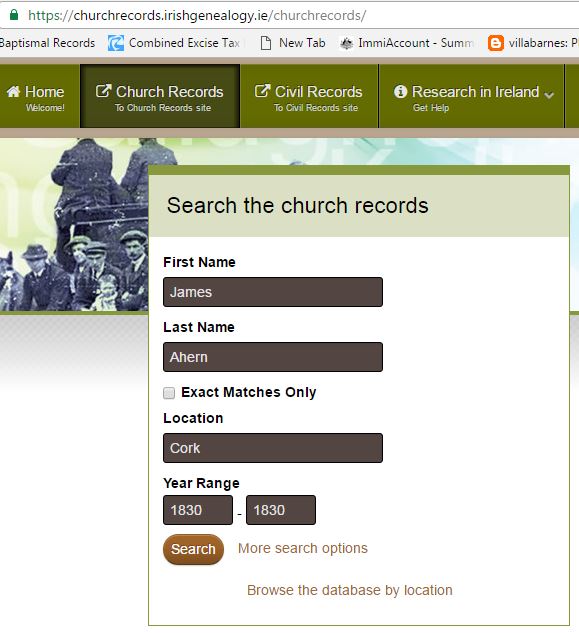  

​Step 2: My search gave me 10 results – 7 baptism and 3 marriage.  For ease of illustrating my example, I filtered out the 3 marriage results, leaving only the 7 baptism results.  (When you’re doing this on your own, feel free to grab all the data you want, but for my example I’m going to limit it so we won’t have an overwhelming amount of data to deal with.)  Just click on the word “Baptism” on the left side of the screen.  Now you should have 7 results of only baptisms.  See the "Before filtering" and "After filtering" illustrations below: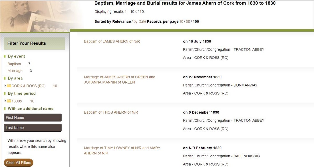

Results before Filtering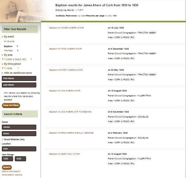

Results after filtering for Baptisms Only

​Step 3: Highlight and select your results to copy them.  I find it easiest to start from the bottom of the list, left mouse click and work my way up to the top of the list.  Once you have your results highlighted click Ctrl + C to copy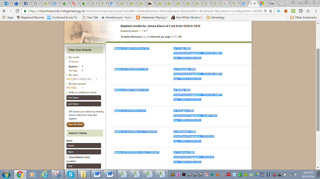

Step 4: Now you are ready to paste into Excel.  To do this, open up a worksheet, put your cursor in cell A1, click the little triangle below the word “Paste” and select "Paste Special – Text."  Click OK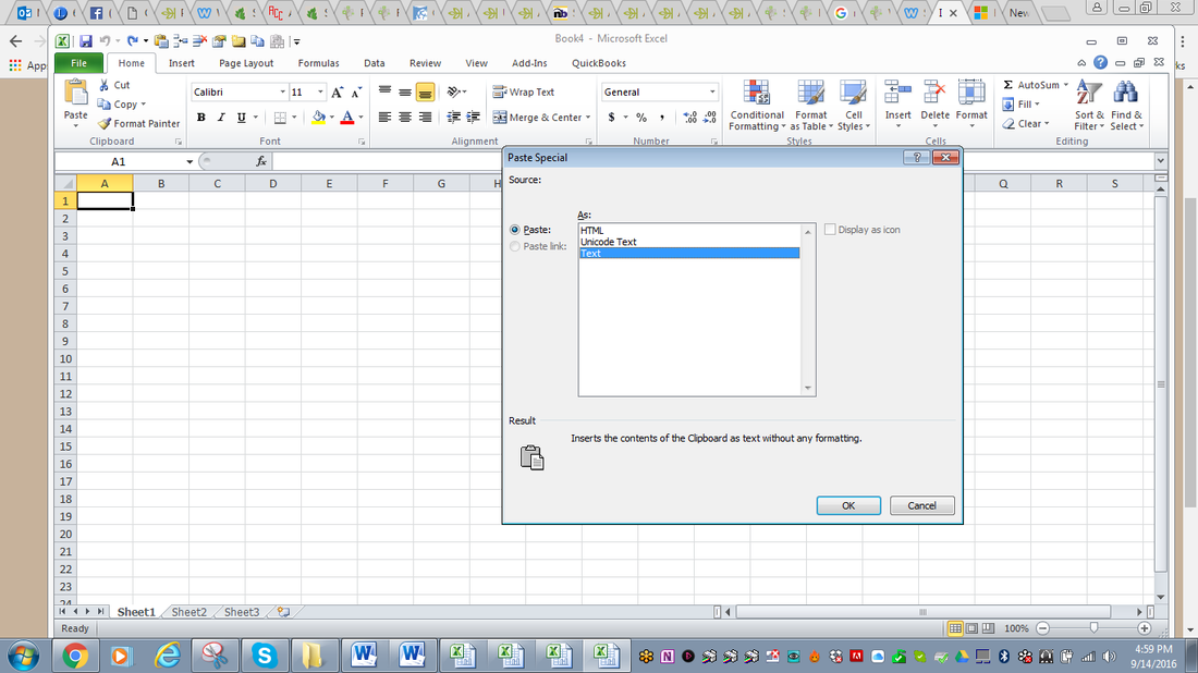

Your worksheet will now look like this:  Note that everything is in Column A.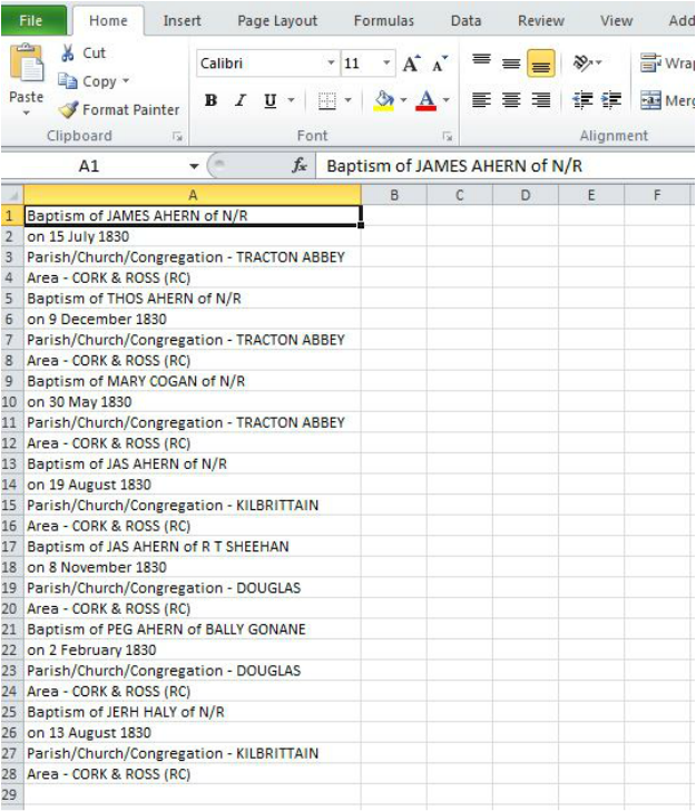

.

---

Step 5: Here’s where the magic happens!  In cell C1, paste the following formula:

=OFFSET($A$1,(ROW()-1)*4+INT((COLUMN()-3)),MOD(COLUMN()-3,1))
​
You can see how that has copied the contents of cell A1 into C1.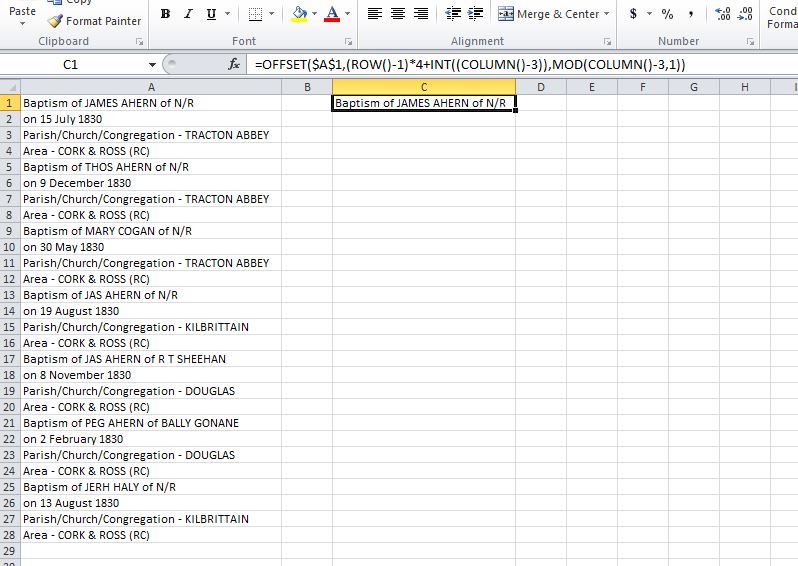

Step 6: Now copy that same formula from C1 and paste it into cells D1, E1 and F1.  Widen each of those columns to fit all the data in them.  See illustration below: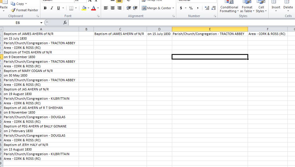

​Step 7: Now copy cells C1-F1 and paste them into cells C2 to C10.  After you click enter, your worksheet should look like this: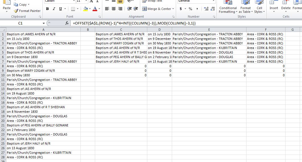

You can see that there are 0s in rows 8-10.  This is because we only have 7 sets of records. (I really didn't need to copy all the way down to C10, but I did just to show you that you can paste more than you need and avoid having to mentally calculate exactly what you need.)


​Step 8: Notice in the image above that the contents of the cells in the worksheet looks like text, but you can see in the function box that it is still a formula.  You need to do one more step to turn these cells into true text.  Click on the grey square in the upper left corner of the worksheet to highlight the entire worksheet.  Click Ctrl + C to copy everything.  In a new worksheet, (ie Sheet2) click on cell A1, click the triangle below the word “Paste” and select “Paste Special – Values.”  This turns all the formulas into text.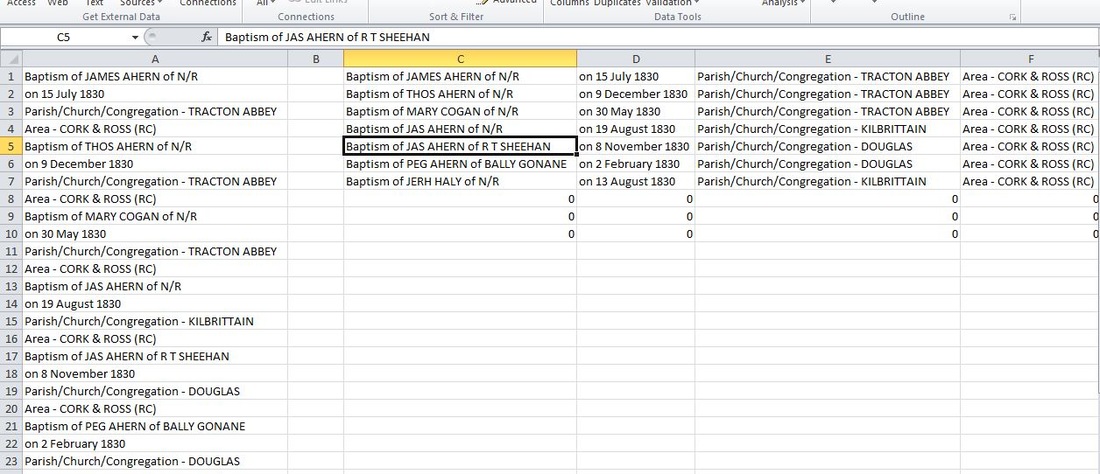  

You can see in the function box that cell C5 now contains text, not a formula.  Perfect!

Then you can use “Text to columns” on the Data tab to split the data in Columns C through F to separate the various words into separate columns as you desire.  If you need more instructions as to how to separate Text to Columns, check out my Legacy Family Tree Webinars on Spreadsheets at http://familytreewebinars.com/maryroddy  (You'll find Text-to-Columns in my Spreadsheets 201 webinar.)

Now that you know how to import data from a website into Excel and NOT have it all dump into one column, how will you use it?  Let me know in the comments below.


 
A note on the formula you pasted into Cell C1:

=OFFSET($A$1,(ROW()-1)*4+INT((COLUMN()-3)),MOD(COLUMN()-3,1))
The 4 in this formula, indicates that 4 rows of data make one record set.  If your data set is a different number of rows, you would need to adjust the formula.   

According to the Microsoft support website: 

"This formula can be interpreted as
OFFSET($A$1,(ROW()-f_row)*rows_in_set+INT((COLUMN()-f_col)/col_in_set), MOD(COLUMN()-f_col,col_in_set))
where:
f_row = row number of this offset formula
f_col = column number of this offset formula
rows_in_set = number of rows that make one record of data
col_in_set = number of columns of data"[i]


[i] Microsoft Support website at https://support.microsoft.com/en-us/kb/214024